VGG-16은 ILSVRC 2014에서 준우승한 합성곱 신경망 모델이다. 옥스포드 대학의 연구팀 VGG(Visual Geometry Group)에서 개발했다. 동일한 대회에서 우승한 구글넷(GoogLeNet)의 인식 오류율은 약 6%로, 인식 오류율이 7%인 VGG-16보다 더 우수한 성능을 보였지만, VGG-16은 이후 연구에 더 많이 활용됐다.
구글넷은 인셉션 모듈(Inception module)을 사용하여 다양한 필터 크기와 풀링 작업으로 병렬 합성곱 연산을 수행한다. 이 방식은 전역 특징과 지역 특징을 모두 포착하여 성능을 높일 수 있다. 그러나 복잡한 구조로 인해 VGG-16과 같이 상대적으로 간단한 구조의 모델만큼 활용되지는 않았다.
1. AlexNet과 VGG-16
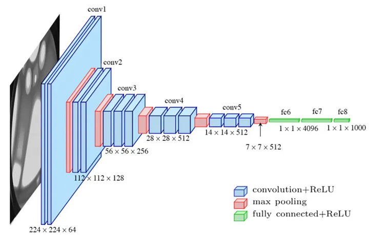
VGG-16은 알렉스넷과 동일하게 합성곱, ReLU, 풀링, 완전 연결 계층을 사용해 구조를 설계했지만, 합성곱 계층의 필터 크기가 다르고 더 많은 계층이 사용되었다.
알렉스넷의 첫 번째 합성곱 계층은 11 x 11 크기의 필터를 적용하고 두 번째는 5 x 5 크기의 필터를 적용했다. 알렉스넷은 비교적 큰 크기의 필터를 사용해 수용 영역(Receptive Field, RF)를 넓게 확보했지만, VGG-16은 3 x 3 필터를 적용해 이미지 특징을 더 정확하게 분석하는 방법을 선택했다.
RF가 크다면 노드가 한 번에 바라보는 이미지의 영역이 커지므로 전역 특징(Global Features)을 더 효율적으로 학습할 수 있지만, 반대로 가장자리(edge)나 모서리(corner)와 같은 낮은 수준의 지역 특징(Local Features)을 학습하는 데 어려움을 겪는다.
VGG-16은 3 x 3필터를 여러 번 적용해 7 x 7 필터를 대신했다. 8 x 8 영역에 stride 1로 7 x 7 필터를 한 번 적용한 것과 3 x 3 필터를 3번 적용한 것은 둘 다 동일하게 2 x 2 크기의 특성 맵을 만들어내지만 매개변수는 49개와 27개로 후자가 더 적다.
또한 작은 필터를 여러 번 적용하면 그만큼 활성화 함수도 여러 번 적용하게 되므로 비선형성을 더 많이 확보하여 모델의 표현력이 높아진다.
2. 모델 구조 및 데이터 시각화
소규모 개와 고양이 데이터셋을 활용해 사전 학습된 VGG-16 모델을 미세 조정해본다. 데이터셋의 pet.zip 파일이고 압축을 해제하면 다음과 같은 구조로 디렉터리가 형성되어있다.
pet
⨽ train
⨽ dog
⨽ dog.1.jpg
⨽ ...
⨽ cat
⨽ cat.1.jpg
⨽ ...
⨽ test
⨽ dog
⨽ dog.4001.jpg
⨽ ...
⨽ cat
⨽ cat.4001.jpg
⨽ ...
하이퍼파라미터 선언 및 이미지 변환
- 탐지하려는 객체가 중앙에 위치할 확률이 높으므로 이미지를 256으로 조절한 후 224로 중앙 자르기를 수행해 불필요한 지역 특징을 제거한다.
- 이미지 폴더 데이터셋 클래스(ImageFolder)는 이미지 데이터를 대상으로 하는 데이터셋으로 폴더 구조가 위와 같은 형태로 구성돼 있으면 이미지와 레이블을 자동으로 인식한다.
from torch.utils.data import DataLoader
from torchvision.datasets import ImageFolder
from torchvision import transforms


hyperparams = {
    'batch_size':4,
    'learning_rate':1e-4,
    'epochs':5,
    'transform':transforms.Compose(
        [
            transforms.Resize(256),
            transforms.CenterCrop(224),
            transforms.ToTensor(),
            transforms.Normalize(
                mean=[0.485, 0.456, 0.406],
                std=[0.229, 0.224, 0.225]
            )
        ]
    )
}

train_dataset = ImageFolder(
    root=IMAGE_PATH / 'train',
    transform=hyperparams['transform']
)
test_dataset = ImageFolder(
    root=IMAGE_PATH / 'test',
    transform=hyperparams['transform']
)

train_dataloader = DataLoader(
    dataset=train_dataset,
    batch_size=hyperparams['batch_size'],
    shuffle=True,
    drop_last=True,
)
test_dataloader = DataLoader(
    dataset=test_dataset,
    batch_size=hyperparams['batch_size'],
    shuffle=True,
    drop_last=True,
)
데이터 시각화
- Tensor 객체는 이미지 형태를 (H, W, C)에서 (C, H, W)로 변환하므로 transpose 메서드를 통해 다시 (H, W, C)로 변환한다.
- 정규화 연산으로 인해 이미지 픽셀들이 재조정됐으므로 이를 다시 역순서로 연산을 적용한다.
import numpy as np
from matplotlib import pyplot as plt


mean = [0.485, 0.456, 0.406]
std = [0.229, 0.224, 0.225]

images, labels = next(iter(train_dataloader))
for image, label in zip(images, labels):
  print(image.size()) # (C, H, W)
  image = image.numpy().transpose(1, 2, 0) # (H, W, C)
  image = ((std * image + mean) * 255).astype(np.uint8)

  plt.imshow(image)
  plt.title(train_dataset.classes[int(label)])
  plt.show()
  break
torch.Size([3, 224, 224])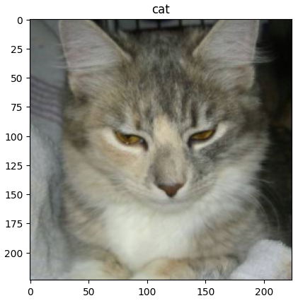
VGG-16 모델 불러오기 및 구조
- pytorch docs를 보면 VGG16_BN_Weights나 VGG13, VGG19 등이 있는데 BN은 배치 정규화를 의미하고 숫자는 레이어의 수를 의미한다.
- 이 방법 말고도 단순히 print(model)을 통해서도 모델 구조를 확인할 수 있다.
from torchvision import models
from torchinfo import summary


model = models.vgg16(weights="VGG16_Weights.IMAGENET1K_V1")
summary(model, input_size=(1, 3, 224, 224))
==========================================================================================
Layer (type:depth-idx) Output Shape Param #
==========================================================================================
VGG [1, 1000] --
├─Sequential: 1-1 [1, 512, 7, 7] --
│ └─Conv2d: 2-1 [1, 64, 224, 224] 1,792
│ └─ReLU: 2-2 [1, 64, 224, 224] --
│ └─Conv2d: 2-3 [1, 64, 224, 224] 36,928
│ └─ReLU: 2-4 [1, 64, 224, 224] --
│ └─MaxPool2d: 2-5 [1, 64, 112, 112] --
│ └─Conv2d: 2-6 [1, 128, 112, 112] 73,856
│ └─ReLU: 2-7 [1, 128, 112, 112] --
│ └─Conv2d: 2-8 [1, 128, 112, 112] 147,584
│ └─ReLU: 2-9 [1, 128, 112, 112] --
│ └─MaxPool2d: 2-10 [1, 128, 56, 56] --
│ └─Conv2d: 2-11 [1, 256, 56, 56] 295,168
│ └─ReLU: 2-12 [1, 256, 56, 56] --
│ └─Conv2d: 2-13 [1, 256, 56, 56] 590,080
│ └─ReLU: 2-14 [1, 256, 56, 56] --
│ └─Conv2d: 2-15 [1, 256, 56, 56] 590,080
│ └─ReLU: 2-16 [1, 256, 56, 56] --
│ └─MaxPool2d: 2-17 [1, 256, 28, 28] --
│ └─Conv2d: 2-18 [1, 512, 28, 28] 1,180,160
│ └─ReLU: 2-19 [1, 512, 28, 28] --
│ └─Conv2d: 2-20 [1, 512, 28, 28] 2,359,808
│ └─ReLU: 2-21 [1, 512, 28, 28] --
│ └─Conv2d: 2-22 [1, 512, 28, 28] 2,359,808
│ └─ReLU: 2-23 [1, 512, 28, 28] --
│ └─MaxPool2d: 2-24 [1, 512, 14, 14] --
│ └─Conv2d: 2-25 [1, 512, 14, 14] 2,359,808
│ └─ReLU: 2-26 [1, 512, 14, 14] --
│ └─Conv2d: 2-27 [1, 512, 14, 14] 2,359,808
│ └─ReLU: 2-28 [1, 512, 14, 14] --
│ └─Conv2d: 2-29 [1, 512, 14, 14] 2,359,808
│ └─ReLU: 2-30 [1, 512, 14, 14] --
│ └─MaxPool2d: 2-31 [1, 512, 7, 7] --
├─AdaptiveAvgPool2d: 1-2 [1, 512, 7, 7] --
├─Sequential: 1-3 [1, 1000] --
│ └─Linear: 2-32 [1, 4096] 102,764,544
│ └─ReLU: 2-33 [1, 4096] --
│ └─Dropout: 2-34 [1, 4096] --
│ └─Linear: 2-35 [1, 4096] 16,781,312
│ └─ReLU: 2-36 [1, 4096] --
│ └─Dropout: 2-37 [1, 4096] --
│ └─Linear: 2-38 [1, 1000] 4,097,000
==========================================================================================
Total params: 138,357,544
Trainable params: 138,357,544
Non-trainable params: 0
Total mult-adds (G): 15.48
==========================================================================================
Input size (MB): 0.60
Forward/backward pass size (MB): 108.45
Params size (MB): 553.43
Estimated Total Size (MB): 662.49
==========================================================================================
Fine Tuning
- 미세 조정을 위해 모든 레이어의 가중치를 동결한다.
- 그런 다음 분류기의 마지막 레이어를 바꿔준다. 새로 생성된 모듈 매개변수의 기본값은 requires_grad=True이기 때문에 학습 시 마지막 계층만 최적화된다.
import torch
from torch import nn
from torch import optim
import torch.nn.functional as F


# 가중치 동결
for param in model.parameters():
    param.requires_grad = False

model.classifier[6] = nn.Linear(4096, len(train_dataset.classes))
device = "cuda" if torch.cuda.is_available() else "cpu"
model = model.to(device)
criterion = nn.CrossEntropyLoss().to(device)
optimizer = optim.SGD(model.parameters(), lr=hyperparams["learning_rate"])from tqdm import tqdm
for epoch in range(hyperparams["epochs"]):
cost = 0.0
for images, classes in tqdm(train_dataloader, desc=f"Epoch {epoch+1}/{hyperparams['epochs']}"):
images = images.to(device)
classes = classes.to(device)
output = model(images)
loss = criterion(output, classes)
optimizer.zero_grad()
loss.backward()
optimizer.step()
cost += loss
cost = cost / len(train_dataloader)
print(f"Epoch : {epoch+1:4d}, Cost : {cost:.3f}")with torch.no_grad():
model.eval()
accuracy = 0.0
for images, classes in test_dataloader:
images = images.to(device)
classes = classes.to(device)
outputs = model(images)
probs = F.softmax(outputs, dim=-1)
outputs_classes = torch.argmax(probs, dim=-1)
accuracy += int(torch.eq(classes, outputs_classes).sum())
print(f"acc@1 : {accuracy / (len(test_dataloader) * hyperparams['batch_size']) * 100:.2f}%")torch.save(model.state_dict(), "../models/VGG16.pt")
print("Saved the model weights")'책 > 파이토치 트랜스포머를 활용한 자연어 처리와 컴퓨터비전 심층학습' 카테고리의 다른 글
| 08 이미지 분류 (4) Grad-CAM (0) | 2024.02.17 |
|---|---|
| 08 이미지 분류 (3) ResNet (0) | 2024.02.15 |
| 08 이미지 분류 (1) AlexNet (0) | 2024.02.13 |
| 07 트랜스포머 (6) T5 (0) | 2024.02.13 |
| 07 트랜스포머 (5) ELECTRA (0) | 2024.02.12 |


