Softmax-with-Loss
크로스 엔트로피를 손실함수로 사용하는 Softmax 계층이다.
계산 그래픈느 다음과 같다.
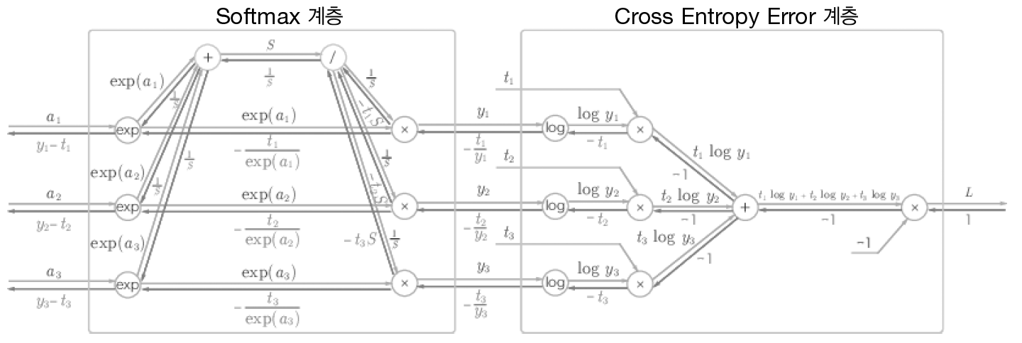
복잡해 보이지만 뒤에서부터 차근차근 이해하면 어렵지 않다.
결론적으로 이 계층의 역전파 결과는 $Y-T$로 깔끔하게 떨어진다. 이러한 부분이 오차역전파가 계산량을 획기적으로 줄여주는 이유이다. 책에서는 이러한 결과가 우연이 아니고 크로스 엔트로피라는 함수가 이렇게 설계되었다고 한다.
이를 클래스로 구현해보자
class SoftmaxWithLoss:
    def __init__(self):
        self.loss = None
        self.y = None
        self.t = None # (one-hot)

    def forward(self, x, t):
        self.t = t
        self.y = softmax(x)
        self.loss = cross_entropy_error(self.y, self.t)
        return self.loss

    def backward(self, dout=1):
        batch_size = self.t.shape[0]
        if self.t.size == self.y.size: # t가 one-hot인 경우
            dx = (self.y - self.t) / batch_size
        else:
            dx = self.y.copy()
            dx[np.arange(batch_size), self.t] -= 1
            dx = dx / batch_size
        return dx
backward 부분에서 역전파가 y - t이므로 t에 해당하는 index만 1을 빼주는 것이다. 그리고 batch_size로 나눠서 데이터 1개당 오차를 앞 계층으로 전파한다.
오차역전파법 구현하기
앞에서 구현한 계층들을 블록 조립하듯이 조립하여 신경망을 구축할 수 있다.
class TwoLayerNet:
    def __init__(self, input_size, hidden_size, output_size, weight_init_std=0.01):
        # 가중치 초기화
        self.params = {}
        self.params['W1'] = weight_init_std * np.random.randn(input_size, hidden_size)
        self.params['b1'] = np.zeros(hidden_size)
        self.params['W2'] = weight_init_std * np.random.randn(hidden_size, output_size)
        self.params['b2'] = np.zeros(output_size)

        # 계층 생성
        self.layers = OrderedDict() # 딕셔너리에 추가한 순서를 기억함
        self.layers['Affine1'] = Affine(self.params['W1'], self.params['b1'])
        self.layers['Relu1'] = Relu()
        self.layers['Affine2'] = Affine(self.params['W2'], self.params['b2'])

        self.lastLayer = SoftmaxWithLoss()
- OrderDict() 을 사용하여 딕셔너리에 추가한 순서를 기억할 수 있다. 이렇게 하면 value들을 하나씩 불러와 간편하게 forward 혹은 backward를 수행할 수 있다.
- SoftmaxWithLoss() 계층을 따로 저장하는 이유는 predict 할 때 필요 없기 때문이다.
    def predict(self, x):
        for layer in self.layers.values():
            x = layer.forward(x)
        return x

    def loss(self, x, t):
        y = self.predict(x)
        return self.lastLayer.forward(y, t)

    def accuracy(self, x, t):
        y = self.predict(x)
        y = np.argmax(y, axis=1)
        if t.ndim != 1: # 정답 레이블이 one-hot인 경우
            t = np.argmax(t, axis=1)
딱히 설명할 것이 없다.
    def gradient(self, x, t):
        # forward
        self.loss(x, t)

        # backward
        dout = 1
        dout = self.lastLayer.backward(dout)

        layers = list(self.layers.values())
        layers.reverse()
        for layer in layers:
            dout = layer.backward(dout)

        grads = {}
        grads['W1'], grads['b1'] = self.layers['Affine1'].dW, self.layers['Affine1'].db
        grads['W2'], grads['b2'] = self.layers['Affine2'].dW, self.layers['Affine2'].db

        return grads
오차역전파를 이용해 gradient를 구한다. 학습할 때 이 메서드를 사용해 gradient를 구하고 가중치 매개변수를 갱신한다.
학습 구현은 중요한게 아니라서 생략!
'책 > 밑바닥부터 시작하는 딥러닝' 카테고리의 다른 글
| 6장 학습 관련 기술들 (2) (0) | 2023.09.20 |
|---|---|
| 6장 학습 관련 기술들 (1) (0) | 2023.09.20 |
| 5장 오차역전파법 (1) (0) | 2023.09.19 |
| 4장 신경망 학습 (2) (0) | 2023.09.14 |
| 4장 신경망 학습 (1) (0) | 2023.09.13 |


